Physics-informed neural operators for the Norne field

01 · Overview

One pipeline, forward and inverse

The Norne example in PhysicsNeMo couples three learned components into a complete reservoir-engineering workflow on a real field model: a Fourier or physics-informed neural operator that advances the black-oil state, a Cluster-Classify-Regress mixture of experts for the well rates, and an adaptive regularised ensemble Kalman inversion that recovers permeability, porosity and fault multipliers from production data.

Forward surrogate (FNO / PINO)

A neural operator maps permeability, porosity, fault multipliers and controls to pressure and saturations at every report step, trained with data and the PDE residual.

Well rates (CCR)

Cluster-Classify-Regress, a mixture of experts built for discontinuous responses, maps the predicted state at the wells to oil, water and gas rates.

Inverse problem (alpha-REKI or ES-MDA)

Adaptive regularised ensemble Kalman inversion, or the ensemble smoother with multiple data assimilation, with covariance localisation, conditions the ensemble on the field history.

Sequential and physics-constrained

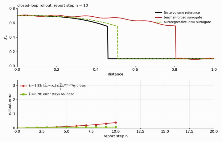
Autoregressive training on the model's own predictions removes the exposure bias of teacher forcing over long rollouts.

02 · Mathematics

What is being learned

In plain words

The neural operator (FNO) learns the map from a permeability field to the pressure and saturation fields over time, from simulator runs.
The physics loss (PINO) also penalises violations of the flow equations, so predictions stay consistent with mass conservation.
The well model (an FNO or CCR) turns the predicted states at the wells into oil, water and gas rates, the part a Peaceman model does in a simulator.
History matching (alpha-REKI or ES-MDA) runs this fast surrogate on whole ensembles to find the fields that reproduce the observed production.

Black-oil mass conservation for water, oil and gas, with dissolved gas and Peaceman well terms.

Autoregressive data loss plus the discretised PDE residual R: the physics-informed neural operator objective.

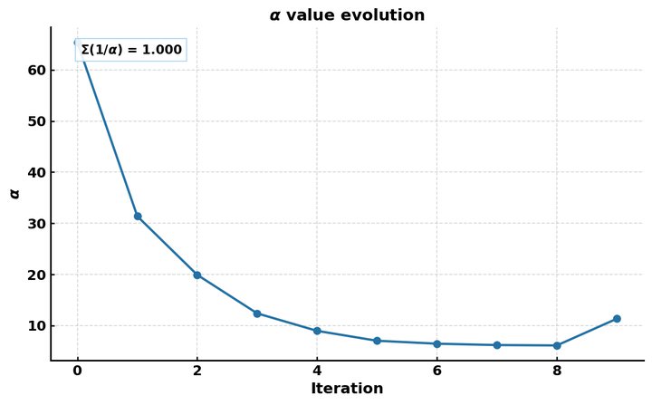
The ensemble Kalman update with the surrogate in place of the simulator. alpha-REKI chooses alpha_i = min(n_d / (2 Phi_i), rho alpha_(i-1)) from the mean data misfit Phi_i and stops when the sum of 1/alpha_i reaches one; ES-MDA uses alpha_i = N_a for N_a assimilations.

03 · The workflow, live

Simulate, train, validate, history-match, verify

The workflow of the paper, end to end, in your browser, on a five-spot with a Gaussian permeability prior. The forward model has two stages, as in the paper: an FNO or a PINO (the same operator trained with the discrete mass-balance residual of the simulator as an extra loss) predicts pressure and water saturation at every report time; the states at each producer are then indexed and passed to the Peaceman well model, learned either by a 1-D FNO over time or by CCR (cluster-classify-regress). The surrogate drives history matching with alpha-REKI or ES-MDA against noisy data from a hidden field; you can also use the mixed-precision simulator itself as the forward model and compare the cost. The simulator then checks the matched model.

1PriorGaussian ln K, six basis functions

2Simulatehidden truth and validation runs

3SurrogateFNO / PINO states, 1-D FNO / CCR wells

4Validateagainst the simulator, with speed-up

5History matchalpha-REKI or ES-MDA

6Verifysimulator on the matched model

Presets

Pick a preset to set the controls for a meaningful experiment; the note says what to watch.

Forward model States model Peaceman well model History matching Ensemble size ES-MDA assimilations Localisation radius, cells (0 = off) Inflation beta (1 = off) Observation noise

Interactive demonstration on a 16 x 16 synthetic model, computed in JavaScript on your CPU. The Norne results on this page come from the full PhysicsNeMo implementation on GPUs.

16 x 16 cells, two-phase, six Gaussian geological parameters, a five-spot (injector in the centre, a producer in each corner), 20 report times of the water cut of every producer, the field oil rate and the injector pressure. The FNO, the PINO and the 1-D FNO were trained offline on 900 runs of the same simulator; their inference runs on this page, and CCR is trained here on the well-cell states of 250 of those runs. With the simulator as the forward model every ensemble member is a full simulation, so the ensemble is capped at 40. Localisation tapers the cross-covariance on the grid with a Gaspari-Cohn function of the distance to the well of each datum and projects the update back onto the six basis functions; with six global parameters and a Gaussian prior the plain update is already well posed, so it is off by default. Inflation (off by default) rescales the ensemble about its mean when its spread falls below half the prior spread; for this Gaussian problem the shrinking spread is the information the data add, so it is a safeguard rather than a necessity. Everything runs in JavaScript on your CPU.

04 · The inverse problem, as a game

Find the hidden channel

The inverse problem of the paper as a game. A sand channel is hidden under an inverted nine-spot (one injector in the centre, eight producers at the corners and edge midpoints), and the simulator reports what the producers saw. Three contestants try to find it with alpha-REKI or ES-MDA, driven by the paper's forward model: an FNO predicts pressure and saturation, and the Peaceman well model is replaced by either a second FNO or CCR (cluster-classify-regress). The first works directly on the 256 grid-cell values of ln K with a Gaussian prior ensemble and no exotic prior at all; the second uses a truncated DCT basis (36 of 256 coefficients); the third a VCAE, a convolutional variational autoencoder trained on channel images, so its updates stay on the channel manifold. You can paint your own guess and send it to the simulator.

1Datasimulator on the hidden field, plus noise

2States FNOln K to p and S at 12 times

3Well modelsecond FNO, or CCR trained live

4Ensemble updatealpha-REKI or ES-MDA, DCT or VCAE prior

5Verifysimulator on the posterior mean

6Scoreyou against the algorithms

Presets

Pick a preset to set the controls for a meaningful experiment; the note says what to watch.

Method Well model Ensemble size ES-MDA assimilations Noise on rates, % (sigma_d) Noise on injector pressure, % Localisation radius, cells (0 = off) Inflation beta (1 = off) Brush Brush size Show Play mode (hide the truth)

Interactive demonstration on a 16 x 16 synthetic model, computed in JavaScript on your CPU. The Norne results on this page come from the full PhysicsNeMo implementation on GPUs.

16 x 16 cells, two-phase. The observations are the oil and water rates of the eight producers and the injector pressure at 12 report times, from the in-browser simulator plus Gaussian noise with a diagonal C_d: sigma_d is the chosen percentage of each value plus a floor (0.01 for rates, 0.02 for pressure). Localisation tapers C_md with a Gaspari-Cohn function of the distance from each cell to the well that measured each datum; it applies to the grid-cell and DCT contestants (for DCT the update is made on the grid and projected back onto the basis); the VCAE's 8 latent variables are global, so it is updated in latent space without a taper. Inflation scales the deviations from the ensemble mean by beta after an update whenever the spread has fallen below half of the prior spread; the log reports the ensemble spread so a collapse is visible. The two FNOs and the VCAE were trained offline on 600 simulator runs and 4,000 channel images; inference, CCR training, the ensemble updates and every simulator run happen on this page, in JavaScript on your CPU. The final check runs the simulator on the posterior mean, on 16 posterior members and on the same 16 members of the starting ensemble.

05 · Movies

Watch it run

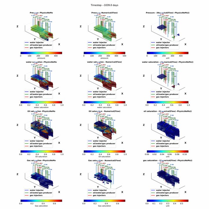
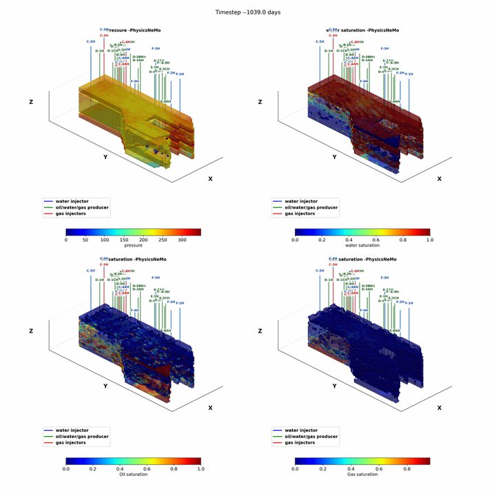
**Forward rollout on Norne**Pressure and saturations predicted by the cascaded PINO-FNO and CCR surrogate against the numerical reference, over the recorded report steps.

**History-matched reservoir model**The best posterior realisation from adaptive regularised ensemble Kalman inversion, run forward through the surrogate.

**Exposure bias in sequential surrogates**A teacher-forced surrogate drifts from the finite-volume reference as its own predictions are fed back, while the autoregressively trained PINO stays bounded: rollout error grows with a Lipschitz constant L = 1.22 and stays bounded for L = 0.78.

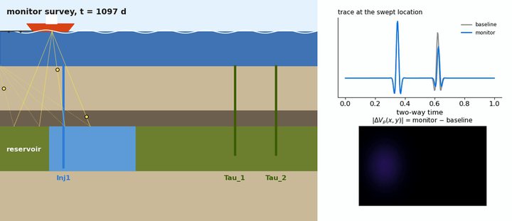
**4D seismic survey**Baseline and monitor surveys over a waterflood and the time-lapse difference that the inversion assimilates alongside production data (schematic).

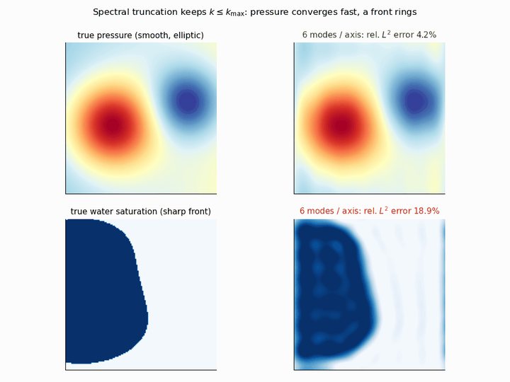
**Spectral truncation in a Fourier neural operator**Keeping k up to k_max modes: the smooth, elliptic pressure converges with few modes, while a sharp saturation front rings.

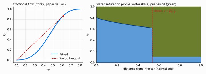
**Buckley-Leverett displacement**Fractional flow with Corey relative permeability, the Welge tangent and the shock it selects; the water saturation profile as water displaces oil.

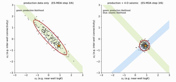
**Ensemble Kalman inversion in parameter space**ES-MDA on a two-parameter problem: production data alone leave a ridge of equally good models; adding 4D seismic collapses the ensemble on the truth.

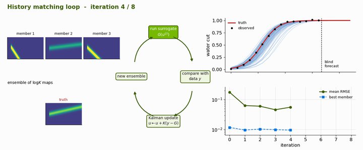
**The history-matching loop**Run the surrogate on every member, compare with the observed data, apply the Kalman update, repeat: water-cut ensemble and misfit per iteration.

06 · Forward results

The surrogate on Norne

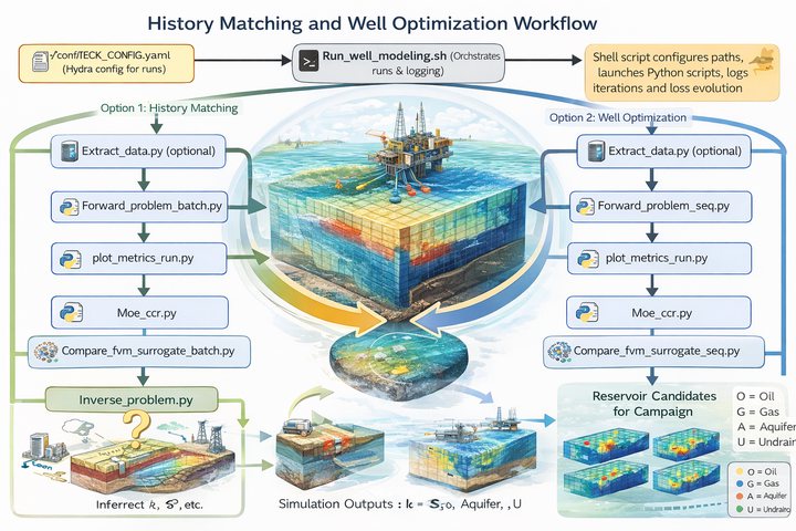
**End-to-end workflow**From the simulation deck to training, forward surrogates, history matching and well optimisation.

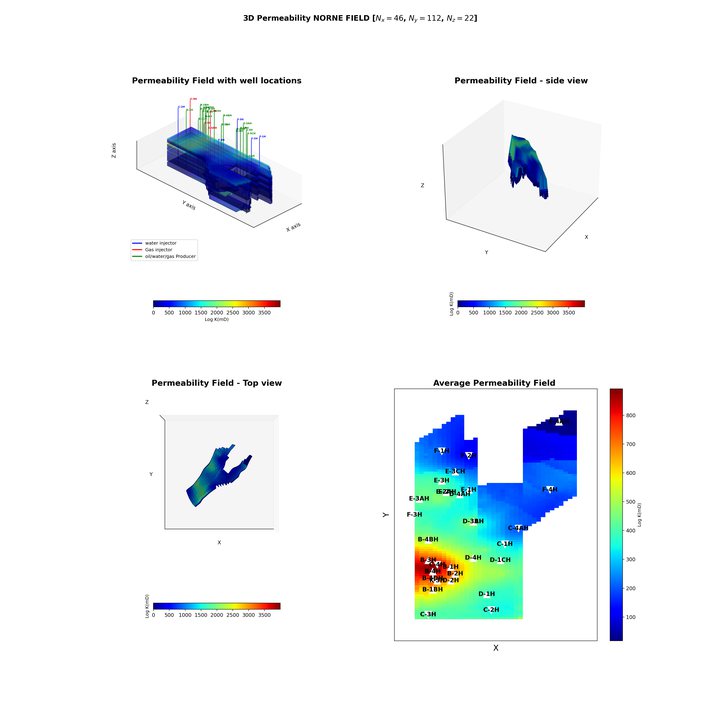
**The Norne field**Permeability of the 46 x 112 x 22 corner-point model with the well locations.

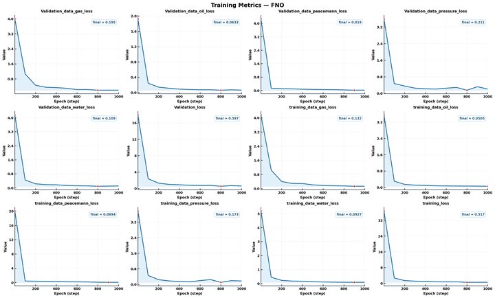
**Training convergence**Training and validation losses of every output head of the FNO surrogate, from MLflow.

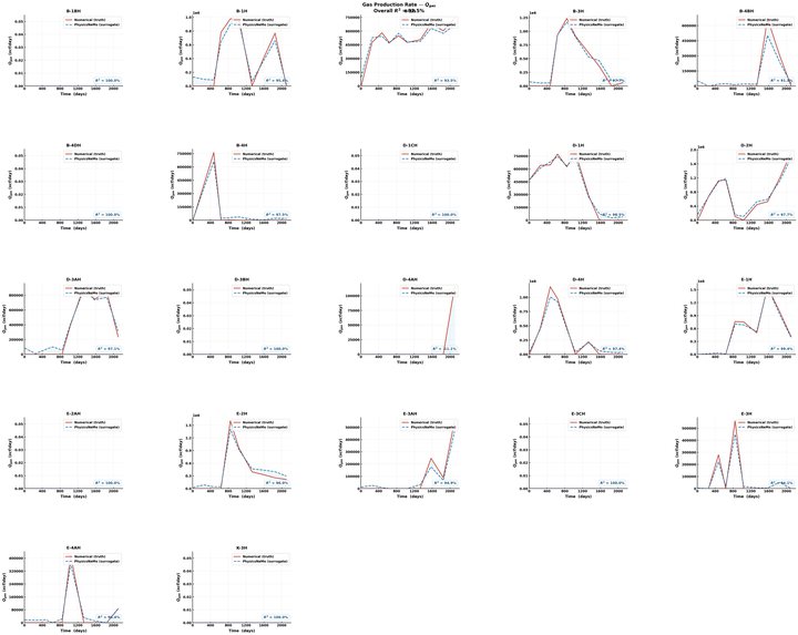
**Gas production rate, every well**Numerical reference against the cascaded PINO-FNO and CCR surrogate.

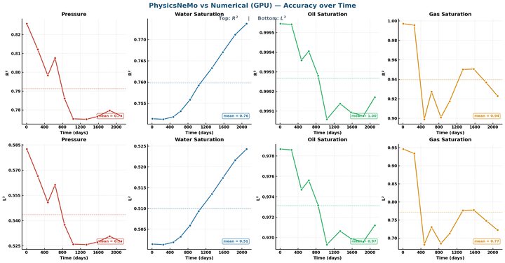
**Accuracy over time**R2 and relative L2 accuracy of pressure and saturations at every report step.

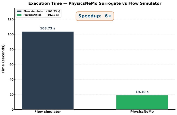
**Execution time**The PhysicsNeMo surrogate against the numerical flow simulator on the same forward run.

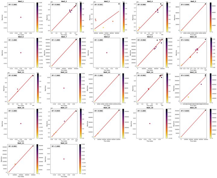
**CCR mixture of experts**Parity plots of the Cluster-Classify-Regress well-rate model against the numerical reference.

07 · Sequential training

Autoregressive against one-to-one training

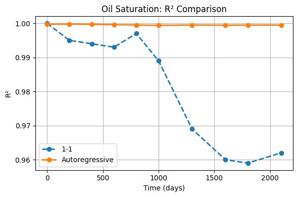
**Oil saturation accuracy over time**One-to-one (teacher-forced) training against autoregressive training: R2 of the rollout.

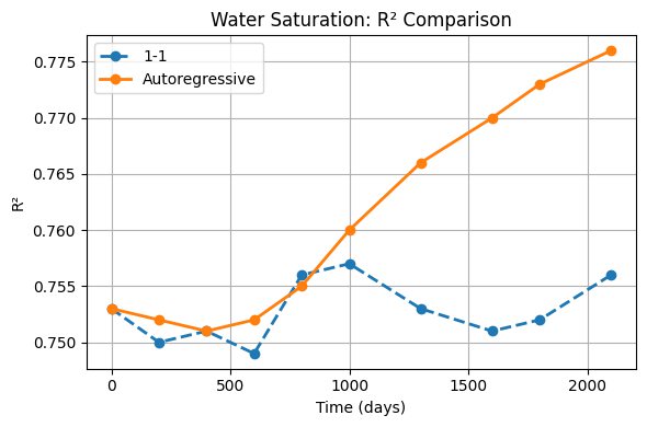
**Water saturation accuracy over time**The autoregressive model keeps its accuracy as the rollout lengthens.

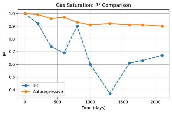
**Gas saturation accuracy over time**Teacher forcing loses accuracy as errors feed back; autoregressive training does not.

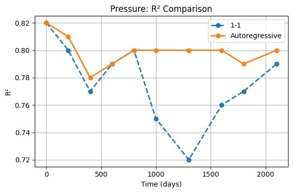
**Pressure accuracy over time**R2 of pressure over the history for both training schemes.

08 · History matching

Conditioning on the field history

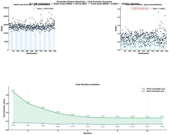
**Misfit reduction**Data misfit of every ensemble member before and after inversion, and its evolution over the iterations.

**Adaptive regularisation**The inflation coefficient chosen at each alpha-REKI iteration; the sum of 1/alpha reaches one at convergence.

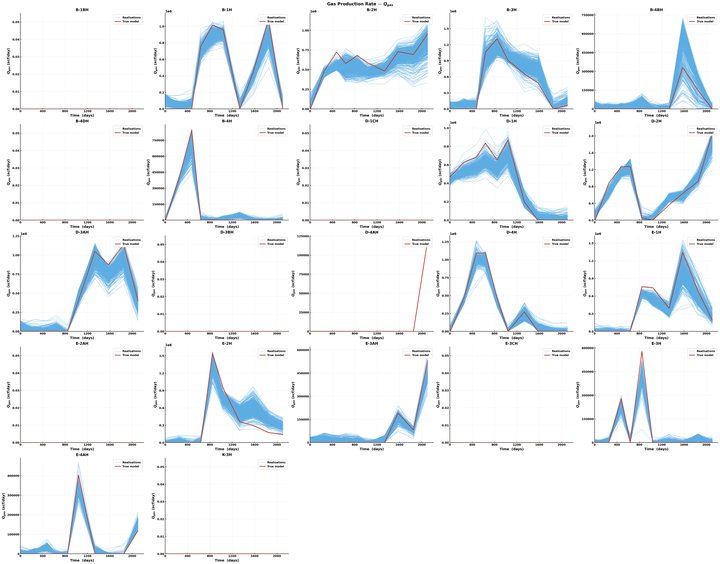
**Prior ensemble**Gas production of the prior ensemble against the observed history.

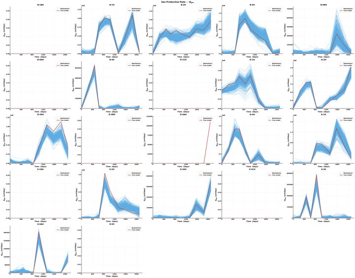
**Posterior ensemble**The same wells after history matching: the ensemble tightens around the observations.

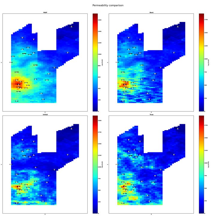
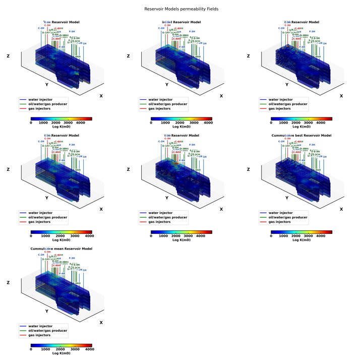
**Recovered permeability**Prior, posterior mean, best and MAP permeability fields.

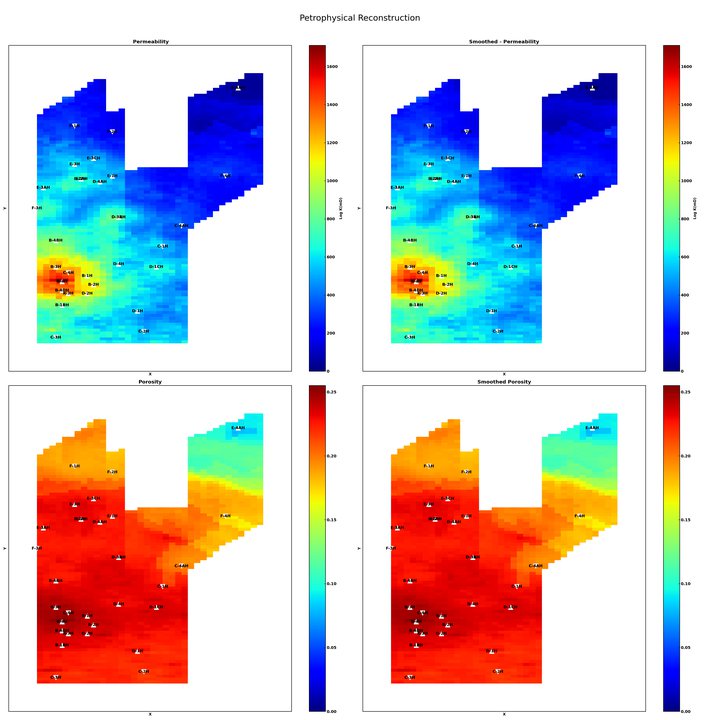
**Posterior mean model**Reconstructed permeability and porosity of the posterior mean.

**P10, P50, P90 models**Percentile reservoir models from the posterior ensemble.

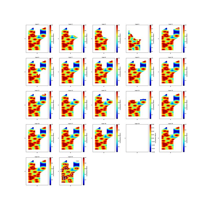
**Covariance localisation**Distance-based localisation of the Kalman gain around each well.

09 · Waterflood demo

Run a waterflood in the browser

A two-phase waterflood, solved in your browser with IMPES: an implicit pressure equation on a heterogeneous permeability field, then an explicit upwind saturation update. This is the kind of forward problem the neural operator learns to replace, at a much smaller scale than Norne. Change the geology and watch the front, the breakthrough time and the recovery change.

water cut at the produceroil recovered

Heterogeneity (std of ln K) Correlation length Oil/water viscosity ratio Geology seed Structure View

A teaching example (IMPES on a 56 x 56 grid), computed in your browser.

56 x 56 cells, quarter five-spot, Corey relative permeability, unit injection rate.

10 · Paper and code

Other featured work

Featured workMixed precision Featured workPhysicsNeMo-Sym HomeClement Etienam

Physics-informed neural operators for the Norne field: forward modelling and history matching